GIS Learn

Land use/land cover maps are used in many areas, such as climate change, natural resource management, and urban/regional planning, and the accuracy of these maps is of critical importance. The OpenStreetMap project has been ongoing since 2004 and provides free geographic and thematic data on a global scale with the help of millions of volunteers. With OpenStreetMap, everyone can contribute to data production, and there is no minimum mapping unit (MMU) in the data produced. However, you can see how spatial resolution affects the accuracy of our analyses in raster data we obtain from other sources. Therefore, we can say that OSM data provides more detailed results in land cover/land use mapping.

However, it is possible to say that there are errors in OSM data. Incorrect thematic information, overlapping features, and temporal and spatial inhomogeneity limit the reliability of OSM data in land cover mapping. OSM data is not comprehensive enough on a global scale. There is a lack of data in some regions.

Schultz et al. (2017) aimed to address this deficiency by using land cover data obtained from open-access satellite images. In this way, it would be possible to produce a highly accurate land cover/land use map on a global scale.

Making a Basic Land Cover Map with OpenStreetMap (OSM)

In OSM, areas or objects are described using tags, which are labels that explain what something is. For example, a tag might say “landuse=forest” to mark an area as a forest or “natural=water” for a lake. The researchers focused on using OSM’s tags to assign land cover categories based on a standard system called Corine Land Cover (CLC), which organizes land into 44 classes (e.g., urban fabric, arable land, forests) across three levels of detail. In this study, they used CLC’s level 2, which has 15 broader categories, to make things manageable.

The OSM database (i.e., table) called “naturals” contains information about natural features and land use. Among the features, polygons are best for mapping land cover.

Polygons with tags related to land cover and land use can include but not limited to,

• landuse (e.g., landuse=forest, landuse=farmland)
• leisure (e.g., leisure=park)
• natural (e.g., natural=water, natural=grassland)
• tourism (e.g., tourism=camp_site)
• waterway (e.g., waterway=riverbank)

By writing an SQL query, it is possible to pull out all relevant polygons from the “naturals” table. This can give us a dataset of tagged areas across the globe. But they specifically focused on Heidelberg, Germany, for their case study.

One of the biggest differences between OSM and CORINE land cover data is that OSM can capture both small and large areas, unlike CLC, which has a minimum mapping unit of 25 hectares.

OSM tags were taken and linked to the CLC level 2 classification system to create a land cover map that could be compared to CLC’s 2012 map. A legend harmonization table shows which OSM tags correspond to which CLC classes. For example:

• CLC Class 1.1 (Urban fabric) was matched to OSM tag “residential.”
• CLC Class 2.1 (Arable land) was matched to OSM tags like “farmland,” “farm,” “greenhouse,” and “horticulture.”
• CLC Class 3.1 (Forests) was matched to OSM tags “forest” and “wood.”
• CLC Class 5.0 (Water bodies) was matched to OSM tags like “water,” “riverbank,” “reservoir,” and “canal.”

However, not every CLC class had a direct OSM tag match. For example, CLC classes like “Artificial non-agricultural vegetated areas” (1.4) or “Heterogeneous agricultural areas” (2.4) do not have clear OSM equivalents. Also, OSM tags can be inconsistent because volunteers might use different tags for similar things (e.g., “wood” vs. “forest”).

After this step, the tagged OSM data can be turned into a map that shows land cover categories based on the CLC system. But this creates a “fractional” map, meaning it only coveres areas where OSM tags were available, leaving gaps where tags were missing.

Filling the Gaps with Satellite Data

Remote sensing means collecting information about the Earth from a distance, usually using satellites that take pictures from space. These pictures (images) show details like forests, cities, or water bodies based on how the land reflects light. It is possible to fill the gaps in the OSM data with the remotely sensed data.

Landsat imagery, thanks to its high temporal resolution, can be effectively used to fill the gaps in the OSM data since it can easily match the different timestamps of the OSM tags. They used a technique called supervised non-parametric classification to figure out the land cover in the gaps. But what does supervised non-parametric mean?

• Supervised: Training a computer to recognize land cover types by showing it examples. In this case, the examples come from the OSM tags.
• Non-parametric: This means the method doesn’t assume the data follows a specific pattern (like a bell curve). It’s flexible and works well for complex landscapes.
• Classification: The computer assigns a land cover category (based on the Corine Land Cover system) to each pixel in the satellite images for the gap areas.

The result of this operation is a continuous coverage Open Land Cover map. There are challenges that we may face during classification; clouds might block the view in the satellite images, or different seasons might change how land looks. Thus, pre-processing is necessary before classifying the images. In addition, matching satellite patterns to Corine Land Cover classes requires careful training to avoid mistakes.

Checking How Good the Map Is

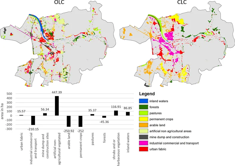
It is necessary to know how accurate the result Open Land Cover map was and whether it was better than the Corine Land Cover map. The researchers used stratified random sampling and several accuracy metrics to evaluate the maps. The results show that OLC map was 87% accurate, while CLC map was 81% accurate, so OLC performed better by 6%. The two maps agreed on land cover for 84% of the study area, meaning they were similar in most places, but Open Land Cover was more detailed, especially in areas with mixed land cover.

Conclusion

OSM’s volunteer contributions made the Open Land Cover flexible and up-to-date, and there are no restrictions on mapping unit or content. Also, using free satellite data and OSM together made the method affordable and accessible. The 87% accuracy (and better performance than CORINE) showed the method’s reliability for applications like urban planning or climate modeling. However, OLC’s tags came from different times, while CLC was all from 2012. This can make comparisons tricky since land cover may change with time. Also, some classes, like “Pastures” and “Shrub/herbaceous vegetation,” are confused, and this reduces accuracy. As an alternative, it is possible to aggregate these classes, but this would reduce detail. Finally, the method provided satisfying accuracy for the selected study area, but the number of OSM tags can be much less in other areas, so the accuracy can significantly decrease.