GIS Learn

Map algebra is a method that allows raster data to be analyzed with mathematical and logical operations in geographic information systems (GIS). Developed by Dr. Dana Tomlin in the 1980s, this method offers a wide range of applications from topographic analysis to hydrological models, from ecological modeling to urban planning. Map algebra works by performing mathematical operations on each cell of raster data and can thus establish relationships between data layers. In Python, we can process raster data with libraries such as Rasterio and GDAL, and perform fast mathematical operations with NumPy. For example, flood risk analyses can be performed by combining a region’s elevation map with precipitation data. These analyses make significant contributions to areas such as environmental management, urban planning and disaster management. Map algebra simplifies data analysis and helps make more effective decisions.

Mathematical Operations with Raster Data

We said that the basis of map algebra is to perform mathematical operations with the values ​​in each cell of raster data. In these mathematical operations, another raster data can be used, or a fixed value can be used. In this example, let’s perform mathematical operations using fixed values ​​on DEM data. It is quite easy to perform mathematical operations with Python. First, let’s import the necessary libraries:

import numpy as np
import matplotlib.pyplot as plt

# Open raster data file
dem_path = '/content/drive/My Drive/Map_Algebra/DEM.tif'

with rasterio.open(dem_path) as src:
  dem = src.read(1)
  profile = src.profile

# Visualize the Digital Terrain Model
plt.figure(figsize=(10,8))
plt.imshow(dem, cmap='terrain')
plt.colorbar(label='Height (m)')
plt.title('DEM')
plt.show()

We specify a constant value to use in mathematical operations;

# Specify a constant value
constant = 10

Now we can add, subtract, multiply and divide using constant.

# Addition
addition = dem + constant

# Subtraction
subtraction = dem - constant

# Multiplication
multiplication = dem * constant

# Division
division = dem / constant

The results of these operations were recorded in the relevant variables. If we want to save them, first let’s specify the file path in our Drive;

# Save the results
output_path = '/content/drive/My Drive/Map_Algebra/'

Now we will write the necessary code to save each result map to our Drive using this file path;

with rasterio.open(output_path + 'addition.tif', 'w', **profile) as dst:
  dst.write(addition, 1)

with rasterio.open(output_path + 'subtraction.tif', 'w', **profile) as dst:
  dst.write(subtraction, 1)

with rasterio.open(output_path + 'multiplication.tif', 'w', **profile) as dst:
  dst.write(multiplication, 1)

with rasterio.open(output_path + 'division.tif', 'w', **profile) as dst:
  dst.write(division, 1)

Let’s visualize one of the result data as an example;

# Visualize the result of multiplication
plt.figure(figsize=(10,8))
plt.imshow(multiplication, cmap='Grays')
plt.colorbar(label='Height (m)')
plt.title('Result of Multiplying DEM by 10')
plt.xlabel('Longitude')
plt.ylabel('Latitude')
plt.show()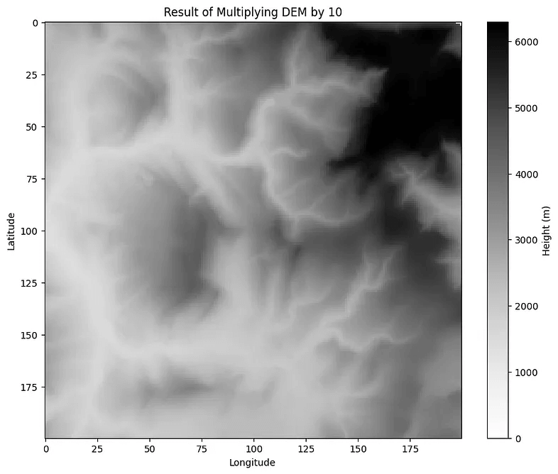

When we compare the legends of these data, we will see the difference. Each pixel value is multiplied by 10.

Logical Operations

Conditional expressions allow making decisions and classifying data based on specific criteria. In Map Algebra, these expressions are applied to raster data to obtain analytical results.

Conditional expressions check whether a cell meets a specific criterion. For example, in elevation data, we can determine cells that are greater than a certain threshold value. We can also use more complex expressions, such as selecting pixels where the elevation is greater than “this” degree and the slope is less than “this” degree, that is, meeting two or more criteria, but let’s keep the example simple and use only the elevation criterion. In this example, we will indicate pixels where the elevation is greater than 300 meters with 1 and pixels where it is less than 300 meters with 0.

First, let’s import numpy;

import numpy as np

We will need rasterio as well, but we already imported that. Additionally, we already opened the raster data file so we will not repeat it. Let’s switch to condition section;

# Conditional expression: Cells with height > 300 are 1, others are 0
conditional_raster = np.where(dem > 300, 1, 0)

# Visualize conditional raster data with Matplotlib
plt.figure(figsize=(10,8))
plt.imshow(conditional_raster, cmap='gray')
plt.colorbar(label='Height (m)')
plt.title('Areas with an altitude greater than 300 meters')
plt.xlabel('Longitude')
plt.ylabel('Latitude')
plt.show()